This post and the covered work were inspired by Tyler Hobb’s post A Generative Approach To Simulating Watercolor Paints. I came across it in April and decided to replicate it from scratch as a first project to build out my own generative art toolkit. This is a walk through of the fun!

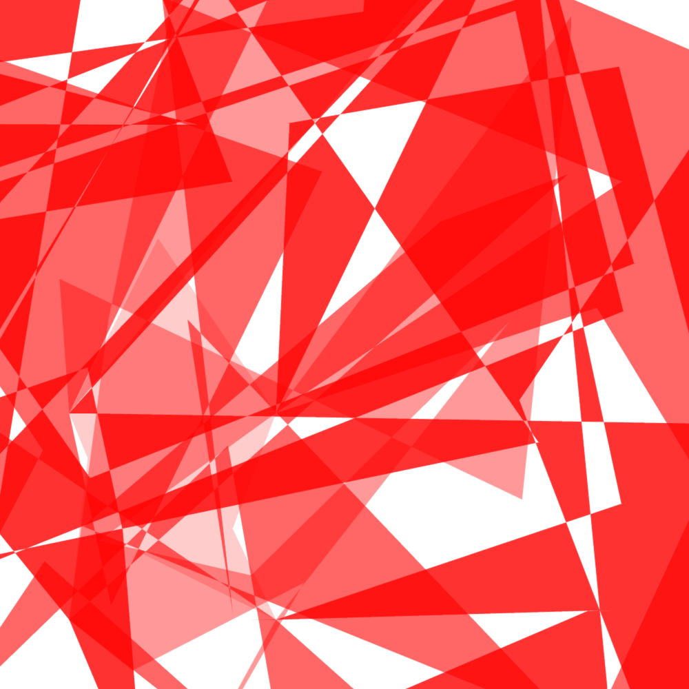
Here's a preview of some results:

In my seven years of programming I have had the most fun in the past few months after discovering generative art. Hopefully you'll see in this guide how fun it can be getting interesting images to look at as a reward for every little challenge you take on. Even the bugs look interesting! If you are a new programmer or unfamiliar with generative art I strongly recommend trying it out! Processing (~Java, (with JavaScript and Python APIs available)), Quil (Clojure), or OpenFrameworks (C++) are powerful tools to get started; you can even try it in your browser at Open Processing. Come share your work with us in /r/generative if you make something, no matter how simple!

I don't go into nearly sufficient detail for anyone to follow along step by step, but I hope to cover the basic ideas and provide links to resources so that if you decide to implement what I describe, you can.

Table of Contents

• An image
• Rendering polygons
  • Choosing a coordinate space
  • Representing polygons
  • Rastering polygons
    • Single sampling polygons
      • Deriving edges
      • Preprocess edges for scanline rendering
      • Shade a pixel
    • Super sampling polygons
  • Using a gpu like a reasonable person
• Making polygons into watercolor
  • A regular n-gon to start
  • Warping our n-gon
    • Finding the polygon center
    • Deriving local strength
  • Subdiving our n-gon
  • Creating a watercolor splotch
    • Using a gpu like a committed person

An image

We will render an image in this guide. To follow along find some library for the language you are using that allows you random access to pixels in an image buffer or on-screen. I used repa in Haskell as a buffer and wrote out to a bitmap.

If you're totally unfamiliar with pixels: they are some tuple of values that represent a color and maybe an opacity. There are many ways of defining color but most common is an rgb color space (there is more to it but for now it doesn't matter). For any given pixel you will have a 4-tuple: (red, green, blue, alpha). Google "color picker" to play around with the values and get a feel for it.

Rendering polygons

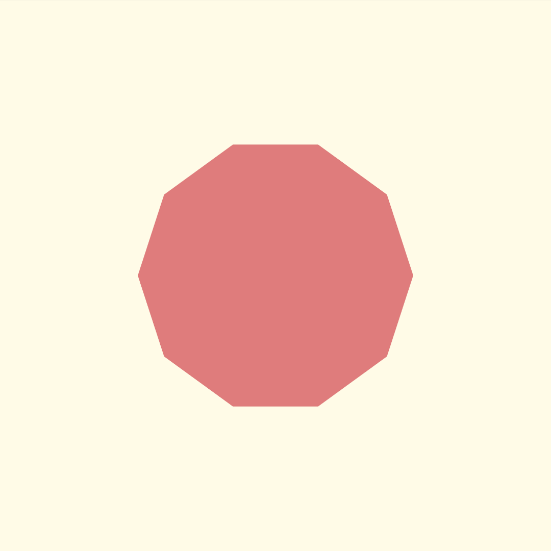
In this chapter we will render a simple square.

Choosing a coordinate space

We need a coordinate space for our polygons to exist in. We will use floating point coordinates because polygons have infinite resolution, even if our output image has a finite one we use integer coordinates for.

This walkthrough will output a square using this coordinate space to keep things simple:

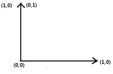
(0.0, 0.0) refers to the bottom left and (1.0, 1.0) refers to the top right.

Representing polygons

First thing, let's get a polygon type to work with. For the purposes of this walkthrough we will use only closed polygons, so my polygon type looks like:

data Point = Point
	{ x :: Double
	, y :: Double }

data Poly = Poly { vertices :: V.Vector Point }

Where I assume that the last vertex connects with the first vertex to close the polygon.

Rastering Polygons

Polygon rastering usually uses some variation of scanline rendering.

If we plot our polygon and imagine a line scanning horizontally across it, we can count the intersections it makes. See this illustration by Vierge Marie:

Look at polygon D and scanline a. Scanline a intersects D twice. If we follow it from left to right and consider at each value of x how many times it has intersected D, we have

• a long section where it has instersected D zero times
• a section where it has intersected D one time
• a section after exiting D where it has intersected D two times

This is the crux of scanline rendering: on pixels where we have intersected the polygon an odd number of times, we shade it as part of the polygon.

Single sampling polygons

To start we will do this for every polygon:

• Derive the edges of the polygon
• Preprocess edges for scanline rendering
• Calculate which edges will be active at each row
• Calculate how many of those edges have been passed at each pixel
• If the count of those edges is odd, shade the pixel

I'll include some Haskell sample code below for guidance because I had a good deal of trouble understanding handwavy guides like this when I first implemented it.

Deriving Edges

edges :: Poly -> V.Vector (Point, Point)
edges Poly { vertices } = V.zip vertices rotated
  where
    rotated = rotateLeft vertices

rotateLeft :: V.Vector a -> V.Vector a
rotateLeft vs = V.snoc (V.head vs) $ V.tail vs

Preprocess edges for scanline rendering

As we travel left to right over each row with a scanline, we need to know some things about our polygon's edges to count how many we intersected so far.

First we need to know: Is this edge intersected by a scan line at height y? a.k.a. Does this edge exist on row y? Look again at polygon D in the scanline diagram and notice that its top right edge is not present in the rows of scanlines b or c. This means we need to know the bottom and top y of each of edge.

Second we need to know: Is this edge to the left of column of x? At what x does the edge intersect the scanline row, and is that x less than the x we're looking at? To do this we must have the edge's slope so we can work backward and find x in terms of y.

These are the questions the type you preprocess your edges into must be able to answer.

You can discard edges with slopes of 0; edges parallel to scanlines don't help.

I used this type:

-- slope in the form of y = mx + b
data Slope
  = Slope { m :: Double
         ,  b :: Double}
  | Vertical Double -- for a vertical line,
		    -- keep a static x

data ScanEdge = ScanEdge
  { high :: Double -- highest y coord of the edge
  , low :: Double -- lowest y coord of the edge
  , slope :: Slope
  }

Which makes the implementation of those two questions look like:

inScanLine :: Double -> ScanEdge -> Bool
inScanLine scanLine ScanEdge {high, low, ..} =
  scanLine >= low && scanLine < high

passedBy :: Point -> ScanEdge -> Bool
passedBy Point {x, y} (ScanEdge {slope, ..}) =
  case slope of
    Slope {m, b} -> (y - b) / m < x
    Vertical staticX -> staticX < x

Shade a pixel

inPoly :: Point -> Poly -> Bool
inPoly point poly = odd $ V.length crossedEdges
  where
    crossed = V.filter (passedBy point) active
    active = V.filter (inScanLine $ y point) allEdges
    allEdges = edges poly

Once you know the pixel is in the polygon, you can shade it however you want!

Super sampling polygons

If you implemented what I've described your square will look crisp, but start rendering some irregular polygons and you will see some janky diagonal lines that look like stairs:

This is because we've been treating pixels as shaded or unshaded for a given polygon; there will necessarily be boundaries on a diagonal line where a pixel passes our test and gets shaded while the neighboring pixel fails the test, creating a stair-like pattern, a result of aliasing.

Earlier I mentioned that polygons are continuous and solving this problem requires treating them that way. When we render a polygon with our scan line algorithm, we sample a continuous space (a grid with infinite resolution where polygons live) and grab a sample of it for each unit of our discrete medium (a grid with finite resolution which is our image). Now we will super sample, meaning we will take more than one sample of the infinite grid per pixel.

Where before we took one sample and decided whether or not to shade the pixel, now we will take four evenly spaced samples per pixel and average the results. For example if three out of our four sub-pixel samples of the polygon are shaded, we color that pixel with 75% opacity.

There are many anti-aliasing methods to choose from, but this simple technique can turn those janky edges pictured above into the much less janky edges pictured below:

Some steps are still visible here where the lines almost become parallel with scanlines (the worst case). You can take your pursuit of smooth polygons much further if that's your taste. See here for a good start.

Using a gpu like a reasonable person

You can follow the rest of this guide with a well written version of the above algorithm; I never had any problems rendering watercolor.

If you are hoping to use the algorithm for bigger things, implementing it in such a way that it can handle the amount of polygons you'll inevitably demand of it in the amount of time you'll want it to is a categorically different endeavor. I spent a great deal of time profiling and re-implementing this algorithm in different languages and never achieved the throughput & latency goals I had.

Luckily you can instead just do the reasonable thing and use a gpu! I won't cover that in this post but the basics are:

1. Tessellate your polygon into triangles because most gpu APIs render only triangles.
2. Write shaders for the graphics card to color the triangles.

See The Book of Shaders for a good introduction and the OpenGL wiki (or the docs for Vulkan if you've got shiny hardware) to get dirty.

Making polygons into watercolor

In this chapter we will make our polygons into water color through a series of deformations of the original polygon.

A regular N-gon to start

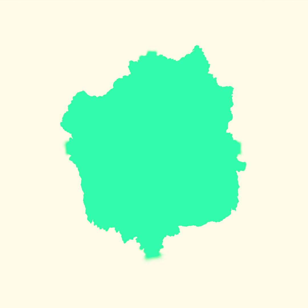
Let's start with a simple regular n-gon. A regular n-gon is a polygon whose n vertices are evenly spaced on the circumference of a circle:

Let's make a function to get a point on the circumference of a circle at a given angle:

circumPoint :: Point -> Double -> Double -> Point
circumPoint Point {x, y} radius angle = Point x' y'
  where
    x' = x + radius * (cos angle)
    y' = y + radius * (sin angle)

Using this we can make a regular n-gon by taking n points on the circumference of our circle.

ngon :: Double -> Int -> Point -> Poly
ngon radius n center = Poly $ V.generate n vertex
  where
    vertex i = circumPoint center radius $ angle i
    angle i = (fromIntegral i) * interval
    interval = (2 * pi) / (fromIntegral n)

Warping our N-gon

Our water color simulation is built using a warp function, which wiggles the vertices of a polygon randomly on a Gaussian distribution.

The algorithm:

1. For each vertex:
   1. Generate a random offset by sampling a Gaussian distribution.
   2. (Optionally) Change the sign of the offset so it always moves the vertex out from the polygon center.
   3. Scale the offset to the local strength.

Our local strength will be the distance between the vertex's surrounding neighbors. So when warping B in vertex set A -> B -> C, our local strength is the distance between A -> C; this should be the upper bound on the vertex's offset.

Finding the polygon center

-- The center of a bounding box around the polygon.
center :: Poly -> Point
center Poly {vertices} = Point x' y'
  where
    x' = (right + left) / 2
    y' = (top + bottom) / 2
    left = V.minimum xs
    right = V.maximum xs
    top = V.maximum ys
    bottom = V.minimum ys
    ys = V.map (y) vertices
    xs = V.map (x) vertices

Deriving local strength

distance :: Point -> Point -> Double
distance p1 p2 = sqrt $ x ^ 2 + y ^ 2
  where
    Point {x, y} = abs $ p1 - p2
    
localStrength :: Poly -> Int -> Double
localStrength (Poly vs) vertex = distance left right
  where
    left = vertices V.! leftIndex
    leftIndex = if vertex - 1 < 0
      then (V.length vertices) - 1
      else vertex - 1
    right = vs V.! ((vertex + 1) % (V.length vs))

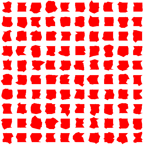
Here's how it ought to look, applying it to the polygon recursively:

Subdividing our N-gon

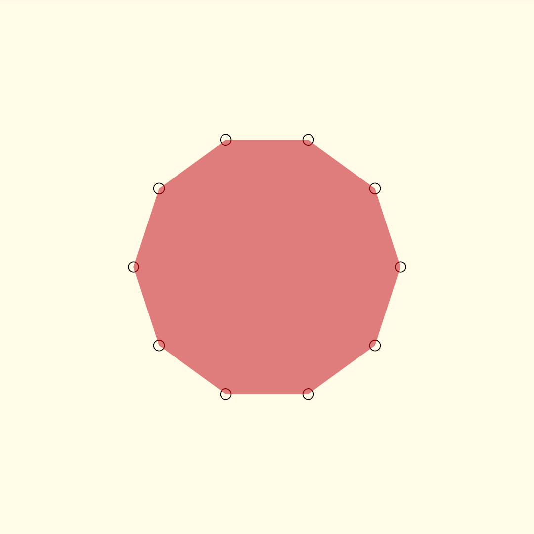
The next core piece of our water color simulation is subdivision of our polygon. For each edge, we want two edges that compose the original edge.

The algorithm:

1. For every edge A -> C
2. Find midpoint B
3. Generate two edges, A -> B and B -> C

midpoint :: Point -> Point -> Point
midpoint (Point x1 y1) (Point x2 y2) = Point x' y'
  where
    x' = x1 + (x2 - x1) / 2
    y' = y1 + (y2 - y1) / 2

subdivideEdges ::  Poly -> Poly
subdivideEdges p@(Poly vs) = Poly vs'
  where
    vs' = V.backpermute ((V.++) vs midpoints) idxs
    idxs = V.generate (2 * (V.length vs)) (place)
    place i =
      if odd i
        then (i `div` 2) + V.length vs
        else i `div` 2
    midpoints = V.map (uncurry midpoint) pairs
    pairs = edges p

The polygon's shape shouldn't change. Here's an illustration of subdividing recursively with vertices highlighted:

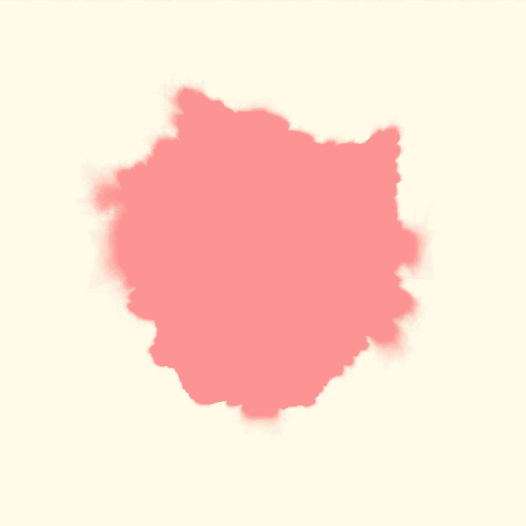
Creating a watercolor splotch

We create layers of the watercolor by combining these two functions and applying them recursively:

Once we have this layer we composite it by:

1. Duplicate it 30-100 times.
2. Decrease opacity to 2-4%.
3. Apply the warp function 4-5 more times to each duplicate.

You will find different results depending on the order in which you apply subdivision and warp functions.

You can also change the spread of different areas by adding to your local strength factor a strength value associated with each vertex in the base polygon. This means some areas will spread out more than others. You can get finer edges by subdividing more often than warping.

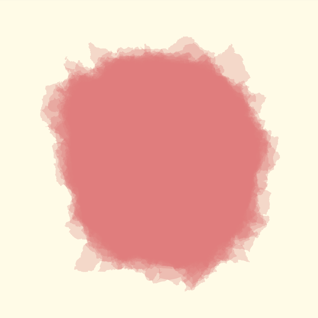
You can also start from the base polygon at each layer instead of working with duplicates of a pre-warped layer. This is my favorite method:

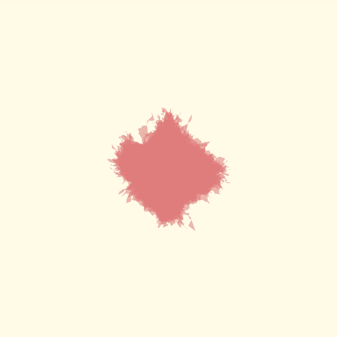
Or you could make the vertex offsets pull inward toward the polygon center instead of outward:

That's it! There are too many variants of these rules to go over, so I'll leave them to explore.

Here's a piece I made with an implementation of this algorithm in my toolkit valora.

Using a gpu like a committed person

This will become slow on cpu if you demand too much even if your implementation is solid. As with most generative art rules it's easier to experiment with it on CPU and if you decide you really want to keep it around you may want to invest in writing shaders to do the work on GPU instead.

If you have questions feel free to ping me on Reddit at /u/roxven!